2.5.2. Surface-based dataset first and second level analysis of a dataset

Full step-by-step example of fitting a GLM (first and second level analysis) in a 10-subjects dataset and visualizing the results.

More specifically:

1. Download an fMRI BIDS dataset with two language conditions to contrast.

2. Project the data to a standard mesh, fsaverage5, aka the Freesurfer template mesh downsampled to about 10k nodes per hemisphere.

3. Run the first level model objects.

4. Fit a second level model on the fitted first level models.

Notice that in this case the preprocessed bold images were already normalized to the same MNI space.

To run this example, you must launch IPython via ipython --matplotlib in a terminal, or use the Jupyter notebook.

2.5.2.1. Fetch example BIDS dataset

We download a simplified BIDS dataset made available for illustrative purposes. It contains only the necessary information to run a statistical analysis using Nistats. The raw data subject folders only contain bold.json and events.tsv files, while the derivatives folder includes the preprocessed files preproc.nii and the confounds.tsv files.

from nistats.datasets import fetch_language_localizer_demo_dataset
data_dir, _ = fetch_language_localizer_demo_dataset()

Here is the location of the dataset on disk.

print(data_dir)

Out:

/home/kshitij/nilearn_data/fMRI-language-localizer-demo-dataset

2.5.2.2. Obtain automatically FirstLevelModel objects and fit arguments

From the dataset directory we automatically obtain the FirstLevelModel objects with their subject_id filled from the BIDS dataset. Moreover, we obtain for each model a dictionary with run_imgs, events and confounder regressors since in this case a confounds.tsv file is available in the BIDS dataset. To get the first level models we only have to specify the dataset directory and the task_label as specified in the file names.

from nistats.first_level_model import first_level_models_from_bids
task_label = 'languagelocalizer'
_, models_run_imgs, models_events, models_confounds = \
    first_level_models_from_bids(
        data_dir, task_label,
        img_filters=[('desc', 'preproc')])

Out:

/home/kshitij/workspace/nistats-org/nistats-repo/nistats-kchawla-pi/nistats/first_level_model.py:861: UserWarning: SliceTimingRef not found in file /home/kshitij/nilearn_data/fMRI-language-localizer-demo-dataset/derivatives/sub-01/func/sub-01_task-languagelocalizer_desc-preproc_bold.json. It will be assumed that the slice timing reference is 0.0 percent of the repetition time. If it is not the case it will need to be set manually in the generated list of models
  img_specs[0])

We also need to get the TR information. For that we use the json sidecar file of the dataset’s functional images.

import os
json_file = os.path.join(data_dir, 'derivatives', 'sub-01', 'func',
                         'sub-01_task-languagelocalizer_desc-preproc_bold.json')
import json
with open(json_file, 'r') as f:
    t_r = json.load(f)['RepetitionTime']

Project fMRI data to the surface: First get fsaverage5.

from nilearn.datasets import fetch_surf_fsaverage
fsaverage = fetch_surf_fsaverage(mesh='fsaverage5')

The projection function simply takes the fMRI data and the mesh. Note that those correspond spatially, as they are both in MNI space.

import numpy as np
from nilearn import surface
from nistats.design_matrix import make_first_level_design_matrix
from nistats.first_level_model import run_glm
from nistats.contrasts import compute_contrast

Empty lists in which we are going to store activation values.

z_scores_right = []
z_scores_left = []
for (fmri_img, confound, events) in zip(
        models_run_imgs, models_confounds, models_events):
    texture = surface.vol_to_surf(fmri_img[0], fsaverage.pial_right)
    n_scans = texture.shape[1]
    frame_times = t_r * (np.arange(n_scans) + .5)

    # Create the design matrix
    #
    # We specify an hrf model containing Glover model and its time derivative.
    # The drift model is implicitly a cosine basis with period cutoff 128s.
    design_matrix = make_first_level_design_matrix(
        frame_times, events=events[0], hrf_model='glover + derivative',
        add_regs=confound[0])

    # Contrast specification
    contrast_values = (design_matrix.columns == 'language') * 1.0 -\
                      (design_matrix.columns == 'string')

    # Setup and fit GLM.
    # Note that the output consists in 2 variables: `labels` and `fit`
    # `labels` tags voxels according to noise autocorrelation.
    # `estimates` contains the parameter estimates.
    # We input them for contrast computation.
    labels, estimates = run_glm(texture.T, design_matrix.values)
    contrast = compute_contrast(labels, estimates, contrast_values,
                                contrast_type='t')
    # We present the Z-transform of the t map.
    z_score = contrast.z_score()
    z_scores_right.append(z_score)

    # Do the left hemipshere exactly in the same way.
    texture = surface.vol_to_surf(fmri_img, fsaverage.pial_left)
    labels, estimates = run_glm(texture.T, design_matrix.values)
    contrast = compute_contrast(labels, estimates, contrast_values,
                                contrast_type='t')
    z_scores_left.append(contrast.z_score())

Individual activation maps have been accumulated in the z_score_left and az_scores_right lists respectively. We can now use them in a group study (one-sample study).

2.5.2.3. Group study

Prepare figure for concurrent plot of individual maps compute population-level maps for left and right hemisphere We directly do that on the value arrays.

from scipy.stats import ttest_1samp, norm
t_left, pval_left = ttest_1samp(np.array(z_scores_left), 0)
t_right, pval_right = ttest_1samp(np.array(z_scores_right), 0)

What we have so far are p-values: we convert them to z-values for plotting.

z_val_left = norm.isf(pval_left)
z_val_right = norm.isf(pval_right)

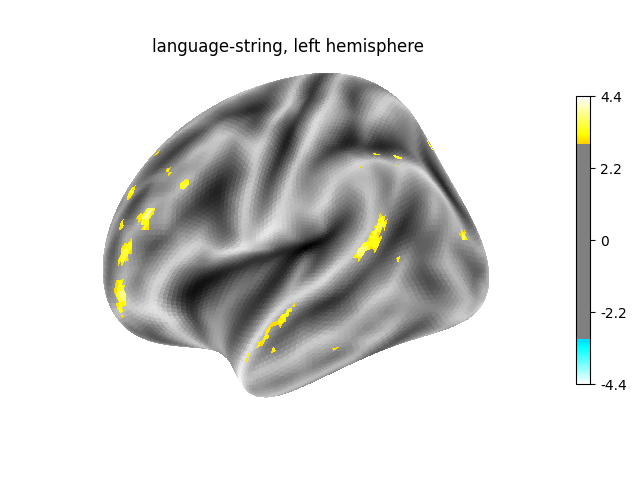
Plot the resulting maps, at first on the left hemipshere.

from nilearn import plotting
plotting.plot_surf_stat_map(
    fsaverage.infl_left, z_val_left, hemi='left',
    title="language-string, left hemisphere", colorbar=True,
    threshold=3., bg_map=fsaverage.sulc_left)

Out:

<Figure size 640x480 with 2 Axes>

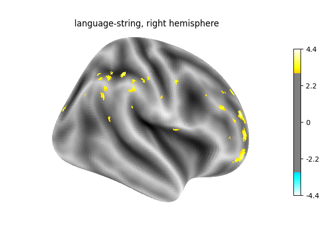
Next, on the right hemisphere.

plotting.plot_surf_stat_map(
    fsaverage.infl_right, z_val_left, hemi='right',
    title="language-string, right hemisphere", colorbar=True,
    threshold=3., bg_map=fsaverage.sulc_right)

plotting.show()