2.2.5. Simple example of two-session fMRI model fitting

Here, we will go through a full step-by-step example of fitting a GLM to experimental data and visualizing the results. This is done on two runs of one subject of the FIAC dataset.

For details on the data, please see:

Dehaene-Lambertz G, Dehaene S, Anton JL, Campagne A, Ciuciu P, Dehaene G, Denghien I, Jobert A, LeBihan D, Sigman M, Pallier C, Poline JB. Functional segregation of cortical language areas by sentence repetition. Hum Brain Mapp. 2006: 27:360–371. http://www.pubmedcentral.nih.gov/articlerender.fcgi?artid=2653076#R11

More specifically:

1. A sequence of fMRI volumes is loaded.

2. A design matrix describing all the effects related to the data is computed.

3. A mask of the useful brain volume is computed.

4. A GLM is applied to the dataset (effect/covariance, then contrast estimation).

Technically, this example shows how to handle two sessions that contain the same experimental conditions. The model directly returns a fixed effect of the statistics across the two sessions.

Create a write directory to work, it will be a ‘results’ subdirectory of the current directory.

from os import mkdir, path, getcwd
write_dir = path.join(getcwd(), 'results')
if not path.exists(write_dir):
    mkdir(write_dir)

2.2.5.1. Prepare data and analysis parameters

Note that there are two sessions.

from nistats import datasets
data = datasets.fetch_fiac_first_level()
fmri_img = [data['func1'], data['func2']]

Create a mean image for plotting purpose.

from nilearn.image import mean_img
mean_img_ = mean_img(fmri_img[0])

The design matrices were pre-computed, we simply put them in a list of DataFrames.

design_files = [data['design_matrix1'], data['design_matrix2']]
import pandas as pd
import numpy as np
design_matrices = [pd.DataFrame(np.load(df)['X']) for df in design_files]

2.2.5.2. GLM estimation

GLM specification. Note that the mask was provided in the dataset. So we use it.

from nistats.first_level_model import FirstLevelModel
fmri_glm = FirstLevelModel(mask_img=data['mask'], minimize_memory=True)

Let’s fit the GLM.

fmri_glm = fmri_glm.fit(fmri_img, design_matrices=design_matrices)

Compute fixed effects of the two runs and compute related images. For this, we first define the contrasts as we would do for a single session.

n_columns = design_matrices[0].shape[1]

def pad_vector(contrast_, n_columns):
    """A small routine to append zeros in contrast vectors"""
    return np.hstack((contrast_, np.zeros(n_columns - len(contrast_))))

Contrast specification

contrasts = {'SStSSp_minus_DStDSp': pad_vector([1, 0, 0, -1], n_columns),
             'DStDSp_minus_SStSSp': pad_vector([-1, 0, 0, 1], n_columns),
             'DSt_minus_SSt': pad_vector([-1, -1, 1, 1], n_columns),
             'DSp_minus_SSp': pad_vector([-1, 1, -1, 1], n_columns),
             'DSt_minus_SSt_for_DSp': pad_vector([0, -1, 0, 1], n_columns),
             'DSp_minus_SSp_for_DSt': pad_vector([0, 0, -1, 1], n_columns),
             'Deactivation': pad_vector([-1, -1, -1, -1, 4], n_columns),
             'Effects_of_interest': np.eye(n_columns)[:5]}

Next, we compute and plot the statistics.

from nilearn import plotting
print('Computing contrasts...')
for index, (contrast_id, contrast_val) in enumerate(contrasts.items()):
    print('  Contrast % 2i out of %i: %s' % (
        index + 1, len(contrasts), contrast_id))
    # estimate the contasts
    # note that the model implictly computes a fixed effect across the two sessions
    z_map = fmri_glm.compute_contrast(
        contrast_val, output_type='z_score')

    # write the resulting stat images to file
    z_image_path = path.join(write_dir, '%s_z_map.nii.gz' % contrast_id)
    z_map.to_filename(z_image_path)

Out:

Computing contrasts...
  Contrast  1 out of 8: SStSSp_minus_DStDSp
/home/kshitij/workspace/nistats-org/nistats-repo/nistats-kchawla-pi/nistats/first_level_model.py:587: UserWarning: One contrast given, assuming it for all 2 runs
  warn('One contrast given, assuming it for all %d runs' % n_runs)
  Contrast  2 out of 8: DStDSp_minus_SStSSp
  Contrast  3 out of 8: DSt_minus_SSt
  Contrast  4 out of 8: DSp_minus_SSp
  Contrast  5 out of 8: DSt_minus_SSt_for_DSp
  Contrast  6 out of 8: DSp_minus_SSp_for_DSt
  Contrast  7 out of 8: Deactivation
  Contrast  8 out of 8: Effects_of_interest
/home/kshitij/workspace/nistats-org/nistats-repo/nistats-kchawla-pi/nistats/contrasts.py:273: UserWarning: Running approximate fixed effects on F statistics.
  warn('Running approximate fixed effects on F statistics.')

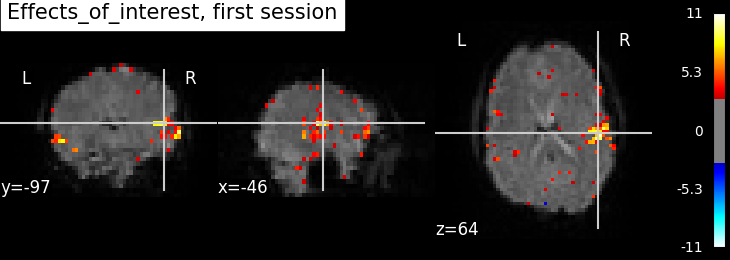
We can then compare session-specific and fixed effects. Here, we compare the activation mas produced from each session separately and then the fixed effects version.

contrast_id = 'Effects_of_interest'

Compute the statistics for the first session.

fmri_glm = fmri_glm.fit(fmri_img[0], design_matrices=design_matrices[0])
z_map = fmri_glm.compute_contrast(
        contrasts[contrast_id], output_type='z_score')
plotting.plot_stat_map(
    z_map, bg_img=mean_img_, threshold=3.0,
    title='%s, first session' % contrast_id)

Out:

<nilearn.plotting.displays.OrthoSlicer object at 0x7f6f143a32e8>

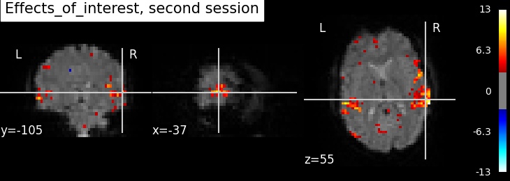
Compute the statistics for the second session.

fmri_glm = fmri_glm.fit(fmri_img[1], design_matrices=design_matrices[1])
z_map = fmri_glm.compute_contrast(
        contrasts[contrast_id], output_type='z_score')
plotting.plot_stat_map(
    z_map, bg_img=mean_img_, threshold=3.0,
    title='%s, second session' % contrast_id)

Out:

<nilearn.plotting.displays.OrthoSlicer object at 0x7f6f14301dd8>

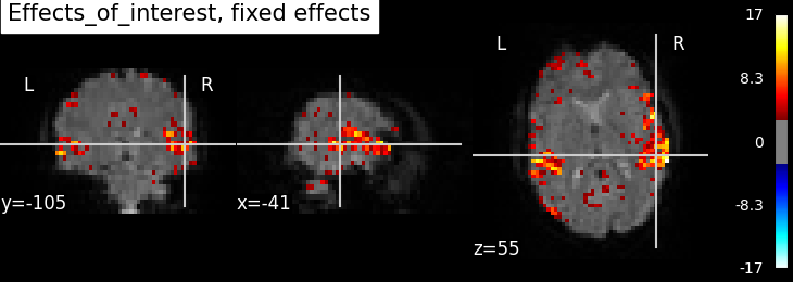
Compute the Fixed effects statistics.

fmri_glm = fmri_glm.fit(fmri_img, design_matrices=design_matrices)
z_map = fmri_glm.compute_contrast(
        contrasts[contrast_id], output_type='z_score')
plotting.plot_stat_map(
    z_map, bg_img=mean_img_, threshold=3.0,
    title='%s, fixed effects' % contrast_id)

plotting.show()

Out:

/home/kshitij/workspace/nistats-org/nistats-repo/nistats-kchawla-pi/nistats/first_level_model.py:587: UserWarning: One contrast given, assuming it for all 2 runs
  warn('One contrast given, assuming it for all %d runs' % n_runs)
/home/kshitij/workspace/nistats-org/nistats-repo/nistats-kchawla-pi/nistats/contrasts.py:273: UserWarning: Running approximate fixed effects on F statistics.
  warn('Running approximate fixed effects on F statistics.')

Not unexpectedly, the fixed effects version displays higher peaks than the input sessions. Computing fixed effects enhances the signal-to-noise ratio of the resulting brain maps.

2.2.5.3. Generating a report

Since we have already computed the FirstLevelModel and and have the contrast, we can quickly create a summary report.

from nistats.reporting import make_glm_report

report = make_glm_report(fmri_glm,
                         contrasts,
                         bg_img=mean_img_,
                         )

Out:

/home/kshitij/workspace/nistats-org/nistats-repo/nistats-kchawla-pi/nistats/first_level_model.py:587: UserWarning: One contrast given, assuming it for all 2 runs
  warn('One contrast given, assuming it for all %d runs' % n_runs)
/home/kshitij/workspace/nistats-org/nistats-repo/nistats-kchawla-pi/nistats/contrasts.py:273: UserWarning: Running approximate fixed effects on F statistics.
  warn('Running approximate fixed effects on F statistics.')

We have several ways to access the report:

# report  # This report can be viewed in a notebook
# report.save_as_html('report.html')
# report.open_in_browser()