2.2.6. First level analysis of a complete BIDS dataset from openneuro

Full step-by-step example of fitting a GLM to perform a first level analysis in an openneuro BIDS dataset. We demonstrate how BIDS derivatives can be exploited to perform a simple one subject analysis with minimal code. Details about the BIDS standard are available at http://bids.neuroimaging.io/. We also demonstrate how to download individual groups of files from the Openneuro s3 bucket.

More specifically:

1. Download an fMRI BIDS dataset with derivatives from openneuro.

2. Extract first level model objects automatically from the BIDS dataset.

3. Demonstrate Quality assurance of Nistats estimation against available FSL. estimation in the openneuro dataset.

4. Display contrast plot and uncorrected first level statistics table report.

To run this example, you must launch IPython via ipython --matplotlib in a terminal, or use the Jupyter notebook.

2.2.6.1. Fetch openneuro BIDS dataset

We download one subject from the stopsignal task in the ds000030 V4 BIDS dataset available in openneuro. This dataset contains the necessary information to run a statistical analysis using Nistats. The dataset also contains statistical results from a previous FSL analysis that we can employ for comparison with the Nistats estimation.

from nistats.datasets import (fetch_openneuro_dataset_index,
                              fetch_openneuro_dataset, select_from_index)

_, urls = fetch_openneuro_dataset_index()

exclusion_patterns = ['*group*', '*phenotype*', '*mriqc*',
                      '*parameter_plots*', '*physio_plots*',
                      '*space-fsaverage*', '*space-T1w*',
                      '*dwi*', '*beh*', '*task-bart*',
                      '*task-rest*', '*task-scap*', '*task-task*']
urls = select_from_index(
    urls, exclusion_filters=exclusion_patterns, n_subjects=1)

data_dir, _ = fetch_openneuro_dataset(urls=urls)

2.2.6.2. Obtain FirstLevelModel objects automatically and fit arguments

From the dataset directory we automatically obtain FirstLevelModel objects with their subject_id filled from the BIDS dataset. Moreover we obtain, for each model, the list of run images and their respective events and confound regressors. Those are inferred from the confounds.tsv files available in the BIDS dataset. To get the first level models we have to specify the dataset directory, the task_label and the space_label as specified in the file names. We also have to provide the folder with the desired derivatives, that in this case were produced by the fmriprep BIDS app.

from nistats.first_level_model import first_level_models_from_bids
task_label = 'stopsignal'
space_label = 'MNI152NLin2009cAsym'
derivatives_folder = 'derivatives/fmriprep'
models, models_run_imgs, models_events, models_confounds = \
    first_level_models_from_bids(
        data_dir, task_label, space_label, smoothing_fwhm=5.0,
        derivatives_folder=derivatives_folder)

Out:

/home/kshitij/workspace/nistats-org/nistats-repo/nistats-kchawla-pi/nistats/first_level_model.py:861: UserWarning: SliceTimingRef not found in file /home/kshitij/nilearn_data/ds000030/ds000030_R1.0.4/uncompressed/sub-10159/func/sub-10159_task-stopsignal_bold.json. It will be assumed that the slice timing reference is 0.0 percent of the repetition time. If it is not the case it will need to be set manually in the generated list of models
  img_specs[0])

Access the model and model arguments of the subject and process events.

model, imgs, events, confounds = (
    models[0], models_run_imgs[0], models_events[0], models_confounds[0])
subject = 'sub-' + model.subject_label

import os
from nistats.utils import get_design_from_fslmat
fsl_design_matrix_path = os.path.join(
    data_dir, 'derivatives', 'task', subject, 'stopsignal.feat', 'design.mat')
design_matrix = get_design_from_fslmat(
    fsl_design_matrix_path, column_names=None)

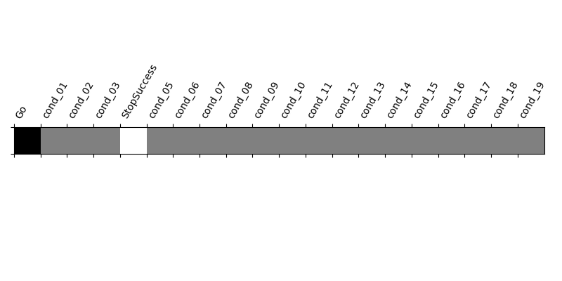
We identify the columns of the Go and StopSuccess conditions of the design matrix inferred from the FSL file, to use them later for contrast definition.

design_columns = ['cond_%02d' % i for i in range(len(design_matrix.columns))]
design_columns[0] = 'Go'
design_columns[4] = 'StopSuccess'
design_matrix.columns = design_columns

2.2.6.3. First level model estimation (one subject)

We fit the first level model for one subject.

model.fit(imgs, design_matrices=[design_matrix])

Out:

FirstLevelModel(drift_model='cosine', drift_order=1, fir_delays=[0],
                high_pass=0.01, hrf_model='glover', mask_img=None,
                memory=Memory(location=None), memory_level=1, min_onset=-24,
                minimize_memory=True, n_jobs=1, noise_model='ar1',
                signal_scaling=True, slice_time_ref=0.0, smoothing_fwhm=5.0,
                standardize=False, subject_label='10159', t_r=2.0,
                target_affine=None, target_shape=None, verbose=0)

Then we compute the StopSuccess - Go contrast. We can use the column names of the design matrix.

z_map = model.compute_contrast('StopSuccess - Go')

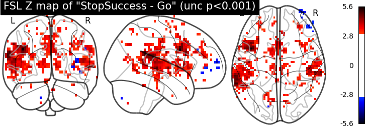
We show the agreement between the Nistats estimation and the FSL estimation available in the dataset.

import nibabel as nib
fsl_z_map = nib.load(
    os.path.join(data_dir, 'derivatives', 'task', subject, 'stopsignal.feat',
                 'stats', 'zstat12.nii.gz'))

from nilearn import plotting
import matplotlib.pyplot as plt
from scipy.stats import norm
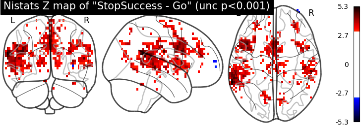
plotting.plot_glass_brain(z_map, colorbar=True, threshold=norm.isf(0.001),
                          title='Nistats Z map of "StopSuccess - Go" (unc p<0.001)',
                          plot_abs=False, display_mode='ortho')
plotting.plot_glass_brain(fsl_z_map, colorbar=True, threshold=norm.isf(0.001),
                          title='FSL Z map of "StopSuccess - Go" (unc p<0.001)',
                          plot_abs=False, display_mode='ortho')
plt.show()

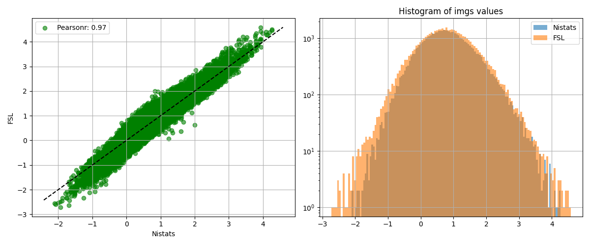
from nistats.reporting import compare_niimgs
compare_niimgs([z_map], [fsl_z_map], model.masker_,
               ref_label='Nistats', src_label='FSL')
plt.show()

• 
• 
• 

Out:

/home/kshitij/workspace/nistats-org/nistats-repo/nistats-kchawla-pi/examples/02_first_level_models/plot_bids_features.py:124: UserWarning: Matplotlib is currently using agg, which is a non-GUI backend, so cannot show the figure.
  plt.show()
/home/kshitij/workspace/nistats-org/nistats-repo/nistats-kchawla-pi/examples/02_first_level_models/plot_bids_features.py:129: UserWarning: Matplotlib is currently using agg, which is a non-GUI backend, so cannot show the figure.
  plt.show()

2.2.6.4. Simple statistical report of thresholded contrast

We display the contrast plot and table with cluster information.

from nistats.reporting import plot_contrast_matrix
plot_contrast_matrix('StopSuccess - Go', design_matrix)
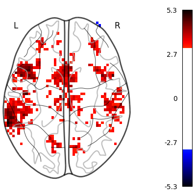
plotting.plot_glass_brain(z_map, colorbar=True, threshold=norm.isf(0.001),
                          plot_abs=False, display_mode='z',
                          figure=plt.figure(figsize=(4, 4)))
plt.show()

• 
• 

Out:

/home/kshitij/workspace/nistats-org/nistats-repo/nistats-kchawla-pi/examples/02_first_level_models/plot_bids_features.py:140: UserWarning: Matplotlib is currently using agg, which is a non-GUI backend, so cannot show the figure.
  plt.show()

We can get a latex table from a Pandas Dataframe for display and publication purposes.

from nistats.reporting import get_clusters_table
print(get_clusters_table(z_map, norm.isf(0.001), 10).to_latex())

Out:

\begin{tabular}{llrrrrl}
\toprule
{} & Cluster ID &     X &     Y &     Z &  Peak Stat & Cluster Size (mm3) \\
\midrule
0  &          1 & -66.0 & -45.0 &  22.0 &   5.307532 &               6300 \\
1  &         1a & -66.0 & -33.0 &  18.0 &   4.668929 &                    \\
2  &         1b & -48.0 & -36.0 &  14.0 &   4.534376 &                    \\
3  &         1c & -57.0 & -48.0 &  10.0 &   4.284222 &                    \\
4  &          2 & -42.0 &  15.0 &  26.0 &   4.918703 &               2520 \\
5  &         2a & -51.0 &   9.0 &  34.0 &   4.715845 &                    \\
6  &         2b & -42.0 &   9.0 &  30.0 &   4.707434 &                    \\
7  &         2c & -57.0 &  12.0 &  38.0 &   4.587956 &                    \\
8  &          3 &  57.0 & -27.0 &   2.0 &   4.692869 &                504 \\
9  &         3a &  66.0 & -27.0 &   2.0 &   3.664250 &                    \\
10 &          4 &  42.0 &   9.0 &  34.0 &   4.461193 &                540 \\
11 &          5 &   6.0 &  18.0 &  34.0 &   4.257986 &               2520 \\
12 &         5a &  -3.0 &  15.0 &  46.0 &   4.078390 &                    \\
13 &         5b &   0.0 &   0.0 &  38.0 &   3.815609 &                    \\
14 &         5c &   3.0 &   9.0 &  50.0 &   3.798387 &                    \\
15 &          6 &   6.0 &   6.0 &  54.0 &   4.208105 &                468 \\
16 &         6a &   6.0 &   3.0 &  62.0 &   3.348351 &                    \\
17 &          7 & -45.0 &  21.0 &   2.0 &   4.190472 &                504 \\
18 &         7a & -54.0 &  21.0 &   6.0 &   3.385929 &                    \\
19 &          8 &  45.0 & -21.0 &  42.0 &   4.163956 &                432 \\
20 &          9 &  63.0 & -24.0 &  30.0 &   4.079389 &                360 \\
21 &         10 & -12.0 &   6.0 &   6.0 &   4.056165 &                792 \\
22 &        10a &  -9.0 &  -3.0 &  10.0 &   3.726486 &                    \\
23 &        10b &  -9.0 &   6.0 &  14.0 &   3.710553 &                    \\
24 &         11 & -27.0 &  45.0 &  18.0 &   4.043724 &                432 \\
25 &         12 &  12.0 & -72.0 &  22.0 &   3.965342 &                360 \\
26 &         13 &   3.0 & -24.0 &  30.0 &   3.950054 &                360 \\
27 &         14 &  33.0 &  42.0 &  34.0 &   3.906274 &                756 \\
28 &        14a &  30.0 &  45.0 &  26.0 &   3.882906 &                    \\
29 &         15 &  51.0 & -30.0 &  14.0 &   3.807061 &                684 \\
\bottomrule
\end{tabular}

2.2.6.5. Generating a report

Using the computed FirstLevelModel and contrast information, we can quickly create a summary report.

from nistats.reporting import make_glm_report

report = make_glm_report(model=model,
                         contrasts='StopSuccess - Go',
                         )

We have several ways to access the report:

# report  # This report can be viewed in a notebook
# report.save_as_html('report.html')
# report.open_in_browser()