2.2.7. Predicted time series and residuals

Here we fit a First Level GLM with the minimize_memory-argument set to False. By doing so, the FirstLevelModel-object stores the residuals, which we can then inspect. Also, the predicted time series can be extracted, which is useful to assess the quality of the model fit.

2.2.7.1. Import modules

from nistats.datasets import fetch_spm_auditory
from nilearn import image
from nilearn import masking
import pandas as pd


# load fMRI data
subject_data = fetch_spm_auditory()
fmri_img = image.concat_imgs(subject_data.func)

# Make an average
mean_img = image.mean_img(fmri_img)
mask = masking.compute_epi_mask(mean_img)

# Clean and smooth data
fmri_img = image.clean_img(fmri_img, standardize=False)
fmri_img = image.smooth_img(fmri_img, 5.)

# load events
events = pd.read_table(subject_data['events'])

2.2.7.2. Fit model

Note that minimize_memory is set to False so that FirstLevelModel stores the residuals. signal_scaling is set to False, so we keep the same scaling as the original data in fmri_img.

from nistats.first_level_model import FirstLevelModel

fmri_glm = FirstLevelModel(t_r=7,
                           drift_model='cosine',
                           signal_scaling=False,
                           mask_img=mask,
                           minimize_memory=False)

fmri_glm = fmri_glm.fit(fmri_img, events)

2.2.7.3. Calculate and plot contrast

from nilearn import plotting

z_map = fmri_glm.compute_contrast('active - rest')

plotting.plot_stat_map(z_map, bg_img=mean_img, threshold=3.1)

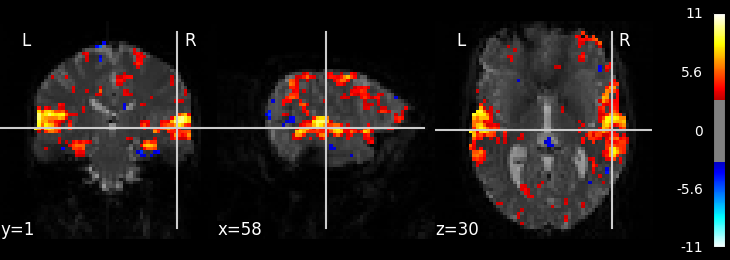
Out:

<nilearn.plotting.displays.OrthoSlicer object at 0x7f6ec4095208>

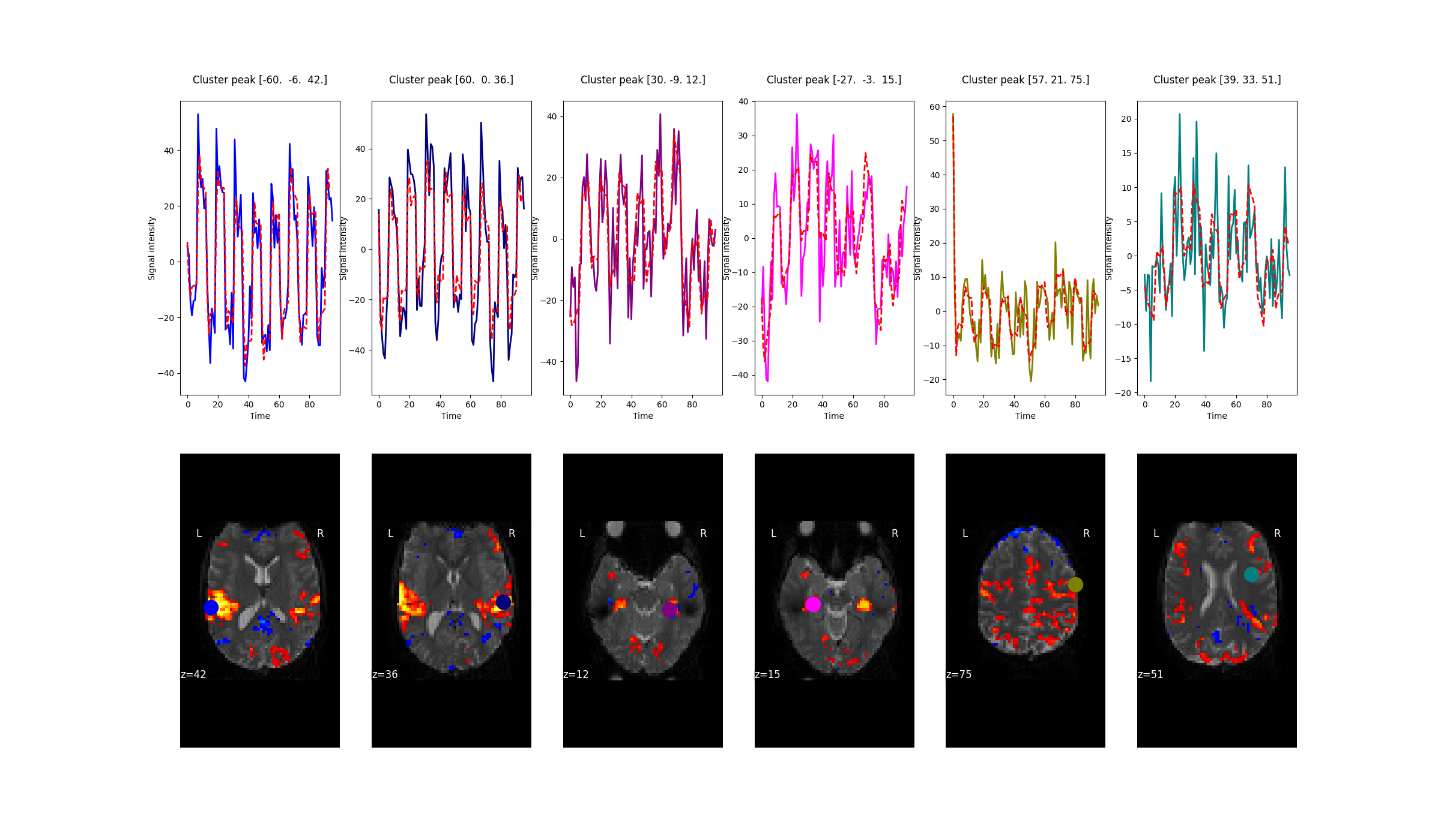
2.2.7.4. Extract the largest clusters

from nistats.reporting import get_clusters_table
from nilearn import input_data

table = get_clusters_table(z_map, stat_threshold=3.1,
                           cluster_threshold=20).set_index('Cluster ID', drop=True)
table.head()

# get the 6 largest clusters' max x, y, and z coordinates
coords = table.loc[range(1, 7), ['X', 'Y', 'Z']].values

# extract time series from each coordinate
masker = input_data.NiftiSpheresMasker(coords)
real_timeseries = masker.fit_transform(fmri_img)
predicted_timeseries = masker.fit_transform(fmri_glm.predicted[0])

2.2.7.5. Plot predicted and actual time series for 6 most significant clusters

import matplotlib.pyplot as plt

# colors for each of the clusters
colors = ['blue', 'navy', 'purple', 'magenta', 'olive', 'teal']
# plot the time series and corresponding locations
fig1, axs1 = plt.subplots(2, 6)
for i in range(0, 6):
    # plotting time series
    axs1[0, i].set_title('Cluster peak {}\n'.format(coords[i]))
    axs1[0, i].plot(real_timeseries[:, i], c=colors[i], lw=2)
    axs1[0, i].plot(predicted_timeseries[:, i], c='r',  ls='--', lw=2)
    axs1[0, i].set_xlabel('Time')
    axs1[0, i].set_ylabel('Signal intensity', labelpad=0)
    # plotting image below the time series
    roi_img = plotting.plot_stat_map(
        z_map, cut_coords=[coords[i][2]], threshold=3.1, figure=fig1,
        axes=axs1[1, i], display_mode='z', colorbar=False, bg_img=mean_img)
    roi_img.add_markers([coords[i]], colors[i], 300)
fig1.set_size_inches(24, 14)

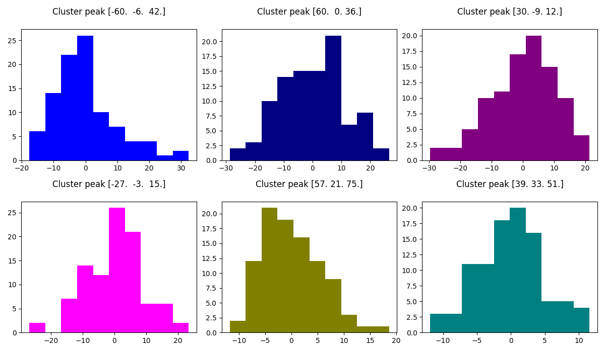
2.2.7.6. Get residuals

resid = masker.fit_transform(fmri_glm.residuals[0])

Out:

/home/kshitij/workspace/nistats-org/nistats-repo/nistats-kchawla-pi/nistats/regression.py:339: FutureWarning: 'resid' from RegressionResults has been deprecated and will be removed. Please use 'residuals' instead.
  FutureWarning,

2.2.7.7. Plot distribution of residuals

Note that residuals are not really distributed normally.

fig2, axs2 = plt.subplots(2, 3)
axs2 = axs2.flatten()
for i in range(0, 6):
    axs2[i].set_title('Cluster peak {}\n'.format(coords[i]))
    axs2[i].hist(resid[:, i], color=colors[i])
    print('Mean residuals: {}'.format(resid[:, i].mean()))

fig2.set_size_inches(12, 7)
fig2.tight_layout()

Out:

Mean residuals: -5.773159728050814e-15
Mean residuals: -0.054243721524977286
Mean residuals: 0.002312283103887758
Mean residuals: 0.01169441049638209
Mean residuals: 0.0023763067961561912
Mean residuals: -0.004646018056754649

2.2.7.8. Plot R-squared

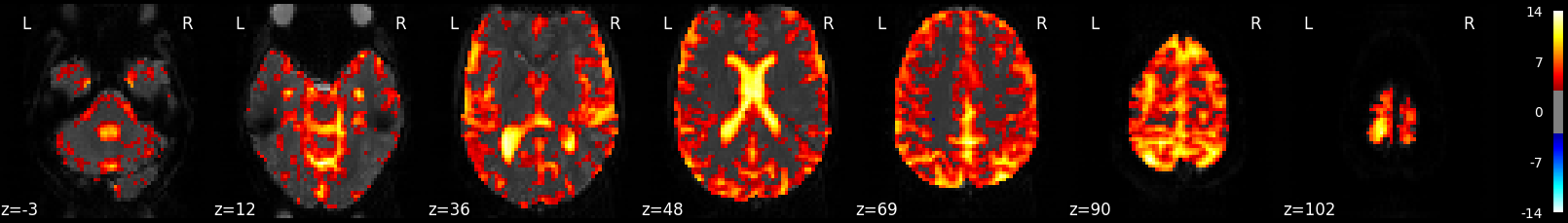
Because we stored the residuals, we can plot the R-squared: the proportion of explained variance of the GLM as a whole. Note that the R-squared is markedly lower deep down the brain, where there is more physiological noise and we are further away from the receive coils. However, R-Squared should be interpreted with a grain of salt. The R-squared value will necessarily increase with the addition of more factors (such as rest, active, drift, motion) into the GLM. Additionally, we are looking at the overall fit of the model, so we are unable to say whether a voxel/region has a large R-squared value because the voxel/region is responsive to the experiment (such as active or rest) or because the voxel/region fits the noise factors (such as drift or motion) that could be present in the GLM. To isolate the influence of the experiment, we can use an F-test as shown in the next section.

plotting.plot_stat_map(fmri_glm.r_square[0],
                       bg_img=mean_img, threshold=.1, display_mode='z', cut_coords=7)

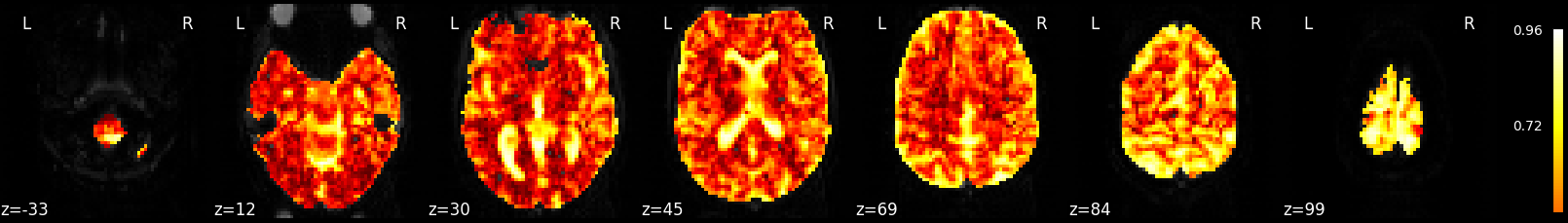
Out:

<nilearn.plotting.displays.ZSlicer object at 0x7f6ec4142e80>

2.2.7.9. Calculate and Plot F-test

The F-test tells you how well the GLM fits effects of interest such as the active and rest conditions together. This is different from R-squared, which tells you how well the overall GLM fits the data, including active, rest and all the other columns in the design matrix such as drift and motion.

import numpy as np

design_matrix = fmri_glm.design_matrices_[0]

# contrast with a one for "active" and zero everywhere else
active = np.array([1 if c == 'active' else 0 for c in design_matrix.columns])

# contrast with a one for "rest" and zero everywhere else
rest = np.array([1 if c == 'rest' else 0 for c in design_matrix.columns])

effects_of_interest = np.vstack((active, rest))
# f-test for rest and activity
z_map_ftest = fmri_glm.compute_contrast(
    effects_of_interest,
    stat_type='F',
    output_type='z_score')

plotting.plot_stat_map(z_map_ftest,
                       bg_img=mean_img, threshold=3.1, display_mode='z', cut_coords=7)

Out:

<nilearn.plotting.displays.ZSlicer object at 0x7f6ec3ed50b8>