2.2.8. Example of surface-based first-level analysis

A full step-by-step example of fitting a GLM to experimental data sampled on the cortical surface and visualizing the results.

More specifically:

1. A sequence of fMRI volumes is loaded.

2. fMRI data are projected onto a reference cortical surface (the FreeSurfer template, fsaverage).

3. A design matrix describing all the effects related to the data is computed.

4. A GLM is applied to the dataset (effect/covariance, then contrast estimation).

The result of the analysis are statistical maps that are defined on the brain mesh. We display them using Nilearn capabilities.

The projection of fMRI data onto a given brain mesh requires that both are initially defined in the same space.

• The functional data should be coregistered to the anatomy from which the mesh was obtained.

• Another possibility, used here, is to project the normalized fMRI data to an MNI-coregistered mesh, such as fsaverage.

The advantage of this second approach is that it makes it easy to run second-level analyses on the surface. On the other hand, it is obviously less accurate than using a subject-tailored mesh.

2.2.8.1. Prepare data and analysis parameters

Prepare the timing parameters.

t_r = 2.4
slice_time_ref = 0.5

Prepare the data. First, the volume-based fMRI data.

from nistats.datasets import fetch_localizer_first_level
data = fetch_localizer_first_level()
fmri_img = data.epi_img

Second, the experimental paradigm.

events_file = data.events
import pandas as pd
events = pd.read_table(events_file)

2.2.8.2. Project the fMRI image to the surface

For this we need to get a mesh representing the geometry of the surface. We could use an individual mesh, but we first resort to a standard mesh, the so-called fsaverage5 template from the FreeSurfer software.

import nilearn
fsaverage = nilearn.datasets.fetch_surf_fsaverage()

The projection function simply takes the fMRI data and the mesh. Note that those correspond spatially, are they are both in MNI space.

from nilearn import surface
texture = surface.vol_to_surf(fmri_img, fsaverage.pial_right)

2.2.8.3. Perform first level analysis

This involves computing the design matrix and fitting the model. We start by specifying the timing of fMRI frames.

import numpy as np
n_scans = texture.shape[1]
frame_times = t_r * (np.arange(n_scans) + .5)

Create the design matrix.

We specify an hrf model containing the Glover model and its time derivative. The drift model is implicitly a cosine basis with a period cutoff at 128s.

from nistats.design_matrix import make_first_level_design_matrix
design_matrix = make_first_level_design_matrix(frame_times,
                                               events=events,
                                               hrf_model='glover + derivative'
                                               )

Setup and fit GLM.

Note that the output consists in 2 variables: labels and fit. labels tags voxels according to noise autocorrelation. estimates contains the parameter estimates. We keep them for later contrast computation.

from nistats.first_level_model import run_glm
labels, estimates = run_glm(texture.T, design_matrix.values)

2.2.8.4. Estimate contrasts

Specify the contrasts.

For practical purpose, we first generate an identity matrix whose size is the number of columns of the design matrix.

contrast_matrix = np.eye(design_matrix.shape[1])

At first, we create basic contrasts.

basic_contrasts = dict([(column, contrast_matrix[i])
                        for i, column in enumerate(design_matrix.columns)])

Next, we add some intermediate contrasts and one contrast adding all conditions with some auditory parts.

basic_contrasts['audio'] = (
    basic_contrasts['audio_left_hand_button_press']
    + basic_contrasts['audio_right_hand_button_press']
    + basic_contrasts['audio_computation']
    + basic_contrasts['sentence_listening'])

# one contrast adding all conditions involving instructions reading
basic_contrasts['visual'] = (
    basic_contrasts['visual_left_hand_button_press']
    + basic_contrasts['visual_right_hand_button_press']
    + basic_contrasts['visual_computation']
    + basic_contrasts['sentence_reading'])

# one contrast adding all conditions involving computation
basic_contrasts['computation'] = (basic_contrasts['visual_computation']
                                  + basic_contrasts['audio_computation'])

# one contrast adding all conditions involving sentences
basic_contrasts['sentences'] = (basic_contrasts['sentence_listening']
                                + basic_contrasts['sentence_reading'])

Finally, we create a dictionary of more relevant contrasts

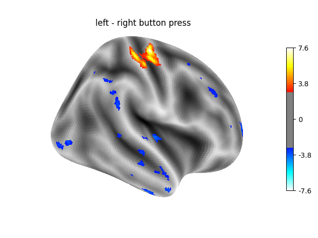
• ‘left - right button press’: probes motor activity in left versus right button presses.

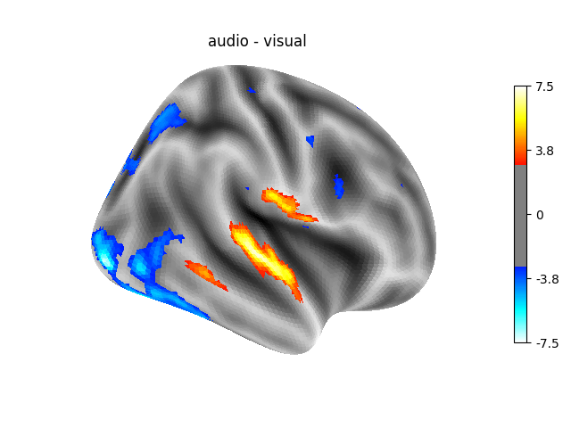
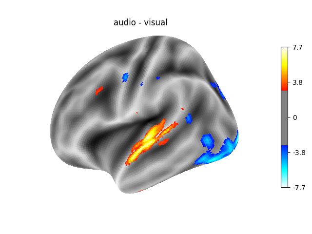
• ‘audio - visual’: probes the difference of activity between listening to some content or reading the same type of content (instructions, stories).

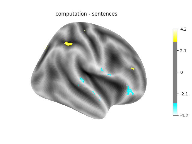
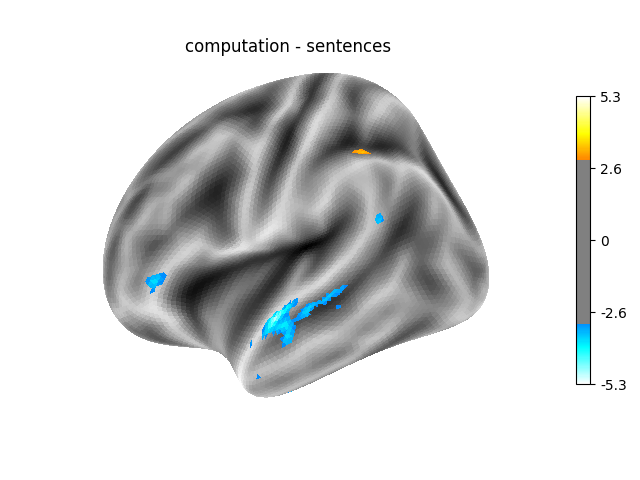
• ‘computation - sentences’: looks at the activity when performing a mental computation task versus simply reading sentences.

Of course, we could define other contrasts, but we keep only 3 for simplicity.

contrasts = {
    'left - right button press': (
        basic_contrasts['audio_left_hand_button_press']
        - basic_contrasts['audio_right_hand_button_press']
        + basic_contrasts['visual_left_hand_button_press']
        - basic_contrasts['visual_right_hand_button_press']
    ),
    'audio - visual': basic_contrasts['audio'] - basic_contrasts['visual'],
    'computation - sentences': (basic_contrasts['computation'] -
                                basic_contrasts['sentences']
    )
}

Let’s estimate the contrasts by iterating over them.

from nistats.contrasts import compute_contrast
from nilearn import plotting

for index, (contrast_id, contrast_val) in enumerate(contrasts.items()):
    print('  Contrast % i out of %i: %s, right hemisphere' %
          (index + 1, len(contrasts), contrast_id))
    # compute contrast-related statistics
    contrast = compute_contrast(labels, estimates, contrast_val,
                                contrast_type='t')
    # we present the Z-transform of the t map
    z_score = contrast.z_score()
    # we plot it on the surface, on the inflated fsaverage mesh,
    # together with a suitable background to give an impression
    # of the cortex folding.
    plotting.plot_surf_stat_map(
        fsaverage.infl_right, z_score, hemi='right',
        title=contrast_id, colorbar=True,
        threshold=3., bg_map=fsaverage.sulc_right)

• 
• 
• 

Out:

Contrast  1 out of 3: left - right button press, right hemisphere
Contrast  2 out of 3: audio - visual, right hemisphere
Contrast  3 out of 3: computation - sentences, right hemisphere

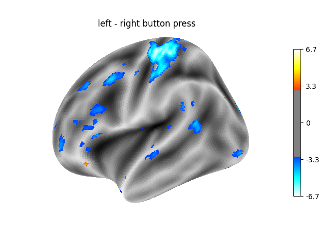
2.2.8.5. Analysing the left hemisphere

Note that re-creating the above analysis for the left hemisphere requires little additional code!

We project the fMRI data to the mesh.

texture = surface.vol_to_surf(fmri_img, fsaverage.pial_left)

Then we estimate the General Linear Model.

labels, estimates = run_glm(texture.T, design_matrix.values)

Finally, we create contrast-specific maps and plot them.

for index, (contrast_id, contrast_val) in enumerate(contrasts.items()):
    print('  Contrast % i out of %i: %s, left hemisphere' %
          (index + 1, len(contrasts), contrast_id))
    # compute contrasts
    contrast = compute_contrast(labels, estimates, contrast_val,
                                contrast_type='t')
    z_score = contrast.z_score()
    # plot the result
    plotting.plot_surf_stat_map(
        fsaverage.infl_left, z_score, hemi='left',
        title=contrast_id, colorbar=True,
        threshold=3., bg_map=fsaverage.sulc_left)

plotting.show()

• 
• 
• 

Out:

Contrast  1 out of 3: left - right button press, left hemisphere
Contrast  2 out of 3: audio - visual, left hemisphere
Contrast  3 out of 3: computation - sentences, left hemisphere