2.3.4. Voxel-Based Morphometry on Oasis dataset

This example uses Voxel-Based Morphometry (VBM) to study the relationship between aging, sex and gray matter density.

The data come from the OASIS project. If you use it, you need to agree with the data usage agreement available on the website.

It has been run through a standard VBM pipeline (using SPM8 and NewSegment) to create VBM maps, which we study here.

2.3.4.1. VBM analysis of aging

We run a standard GLM analysis to study the association between age and gray matter density from the VBM data. We use only 100 subjects from the OASIS dataset to limit the memory usage.

Note that more power would be obtained from using a larger sample of subjects.

# Authors: Bertrand Thirion, <bertrand.thirion@inria.fr>, July 2018
#          Elvis Dhomatob, <elvis.dohmatob@inria.fr>, Apr. 2014
#          Virgile Fritsch, <virgile.fritsch@inria.fr>, Apr 2014
#          Gael Varoquaux, Apr 2014


n_subjects = 100  # more subjects requires more memory

2.3.4.2. Load Oasis dataset

from nilearn import datasets
oasis_dataset = datasets.fetch_oasis_vbm(n_subjects=n_subjects)
gray_matter_map_filenames = oasis_dataset.gray_matter_maps
age = oasis_dataset.ext_vars['age'].astype(float)

Out:

/home/kshitij/miniconda3/envs/nistats-py36-latest/lib/python3.6/site-packages/numpy/lib/npyio.py:2372: VisibleDeprecationWarning: Reading unicode strings without specifying the encoding argument is deprecated. Set the encoding, use None for the system default.
  output = genfromtxt(fname, **kwargs)

Sex is encoded as ‘M’ or ‘F’. Hence, we make it a binary variable.

sex = oasis_dataset.ext_vars['mf'] == b'F'

Print basic information on the dataset.

print('First gray-matter anatomy image (3D) is located at: %s' %
      oasis_dataset.gray_matter_maps[0])  # 3D data
print('First white-matter anatomy image (3D) is located at: %s' %
      oasis_dataset.white_matter_maps[0])  # 3D data

Out:

First gray-matter anatomy image (3D) is located at: /home/kshitij/nilearn_data/oasis1/OAS1_0001_MR1/mwrc1OAS1_0001_MR1_mpr_anon_fslswapdim_bet.nii.gz
First white-matter anatomy image (3D) is located at: /home/kshitij/nilearn_data/oasis1/OAS1_0001_MR1/mwrc2OAS1_0001_MR1_mpr_anon_fslswapdim_bet.nii.gz

Get a mask image: A mask of the cortex of the ICBM template.

gm_mask = datasets.fetch_icbm152_brain_gm_mask()

Resample the images, since this mask has a different resolution.

from nilearn.image import resample_to_img
mask_img = resample_to_img(
    gm_mask, gray_matter_map_filenames[0], interpolation='nearest')

2.3.4.3. Analyse data

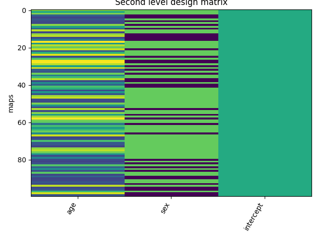
First, we create an adequate design matrix with three columns: ‘age’, ‘sex’, ‘intercept’.

import pandas as pd
import numpy as np
intercept = np.ones(n_subjects)
design_matrix = pd.DataFrame(np.vstack((age, sex, intercept)).T,
                             columns=['age', 'sex', 'intercept'])

Let’s plot the design matrix.

from nistats.reporting import plot_design_matrix

ax = plot_design_matrix(design_matrix)
ax.set_title('Second level design matrix', fontsize=12)
ax.set_ylabel('maps')

Out:

Text(47.097222222222214, 0.5, 'maps')

Next, we specify and fit the second-level model when loading the data and also smooth a little bit to improve statistical behavior.

from nistats.second_level_model import SecondLevelModel
second_level_model = SecondLevelModel(smoothing_fwhm=2.0, mask_img=mask_img)
second_level_model.fit(gray_matter_map_filenames,
                       design_matrix=design_matrix)

Out:

SecondLevelModel(mask_img=<nibabel.nifti1.Nifti1Image object at 0x7f6f14454a58>,
                 memory=Memory(location=None), memory_level=1,
                 minimize_memory=True, n_jobs=1, smoothing_fwhm=2.0, verbose=0)

Estimating the contrast is very simple. We can just provide the column name of the design matrix.

z_map = second_level_model.compute_contrast(second_level_contrast=[1, 0, 0],
                                            output_type='z_score')

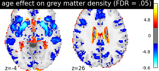
We threshold the second level contrast at uncorrected p < 0.001 and plot it.

from nistats.thresholding import map_threshold
from nilearn import plotting

_, threshold = map_threshold(
    z_map, alpha=.05, height_control='fdr')
print('The FDR=.05-corrected threshold is: %.3g' % threshold)

display = plotting.plot_stat_map(
    z_map, threshold=threshold, colorbar=True, display_mode='z',
    cut_coords=[-4, 26],
    title='age effect on grey matter density (FDR = .05)')
plotting.show()

Out:

The FDR=.05-corrected threshold is: 2.4

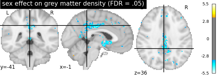
We can also study the effect of sex by computing the contrast, thresholding it and plot the resulting map.

z_map = second_level_model.compute_contrast(second_level_contrast='sex',
                                            output_type='z_score')
_, threshold = map_threshold(
    z_map, alpha=.05, height_control='fdr')
plotting.plot_stat_map(
    z_map, threshold=threshold, colorbar=True,
    title='sex effect on grey matter density (FDR = .05)')

Out:

<nilearn.plotting.displays.OrthoSlicer object at 0x7f6f13ccda58>

Note that there does not seem to be any significant effect of sex on grey matter density on that dataset.

2.3.4.4. Generating a report

It can be useful to quickly generate a portable, ready-to-view report with most of the pertinent information. This is easy to do if you have a fitted model and the list of contrasts, which we do here.

from nistats.reporting import make_glm_report

icbm152_2009 = datasets.fetch_icbm152_2009()
report = make_glm_report(model=second_level_model,
                         contrasts=['age', 'sex'],
                         bg_img=icbm152_2009['t1'],
                         )

We have several ways to access the report:

# report  # This report can be viewed in a notebook
# report.save_as_html('report.html')
# report.open_in_browser()