2.3.6. Example of generic design in second-level models

This example shows the results obtained in a group analysis using a more complex contrast than a one- or two-sample t test. We use the [left button press (auditory cue)] task from the Localizer dataset and seek association between the contrast values and a variate that measures the speed of pseudo-word reading. No confounding variate is included in the model.

# Author: Virgile Fritsch, Bertrand Thirion, 2014 -- 2018
#         Jerome-Alexis Chevalier, 2019

At first, we need to load the Localizer contrasts.

from nilearn import datasets
n_samples = 94
localizer_dataset = datasets.fetch_localizer_contrasts(
    ['left button press (auditory cue)'], n_subjects=n_samples)

Out:

/home/kshitij/miniconda3/envs/nistats-py36-latest/lib/python3.6/site-packages/numpy/lib/npyio.py:2372: VisibleDeprecationWarning: Reading unicode strings without specifying the encoding argument is deprecated. Set the encoding, use None for the system default.
  output = genfromtxt(fname, **kwargs)

Let’s print basic information on the dataset.

print('First contrast nifti image (3D) is located at: %s' %
      localizer_dataset.cmaps[0])

Out:

First contrast nifti image (3D) is located at: /home/kshitij/nilearn_data/brainomics_localizer/brainomics_data/S01/cmaps_LeftAuditoryClick.nii.gz

we also need to load the behavioral variable.

tested_var = localizer_dataset.ext_vars['pseudo']
print(tested_var)

Out:

[b'15.0' b'16.0' b'14.0' b'19.0' b'16.0' b'18.0' b'22.0' b'19.0' b'17.0'
 b'15.0' b'10.0' b'21.0' b'17.0' b'21.0' b'n/a' b'14.0' b'22.0' b'17.0'
 b'23.0' b'15.0' b'15.0' b'18.0' b'17.0' b'18.0' b'20.0' b'27.0' b'18.0'
 b'16.0' b'18.0' b'17.0' b'19.0' b'22.0' b'15.0' b'16.0' b'21.0' b'20.0'
 b'12.0' b'n/a' b'19.0' b'19.0' b'16.0' b'22.0' b'23.0' b'14.0' b'24.0'
 b'22.0' b'20.0' b'25.0' b'23.0' b'15.0' b'12.0' b'16.0' b'20.0' b'18.0'
 b'14.0' b'14.0' b'18.0' b'20.0' b'19.0' b'14.0' b'27.0' b'n/a' b'13.0'
 b'17.0' b'19.0' b'19.0' b'14.0' b'17.0' b'15.0' b'15.0' b'14.0' b'20.0'
 b'16.0' b'15.0' b'15.0' b'15.0' b'19.0' b'17.0' b'14.0' b'15.0' b'n/a'
 b'20.0' b'15.0' b'17.0' b'18.0' b'17.5' b'n/a' b'15.0' b'23.0' b'12.0'
 b'16.0' b'13.0' b'25.0' b'21.0']

It is worth to do a auality check and remove subjects with missing values.

import numpy as np
mask_quality_check = np.where(tested_var != b'n/a')[0]
n_samples = mask_quality_check.size
contrast_map_filenames = [localizer_dataset.cmaps[i]
                          for i in mask_quality_check]
tested_var = tested_var[mask_quality_check].astype(float).reshape((-1, 1))
print("Actual number of subjects after quality check: %d" % n_samples)

Out:

Actual number of subjects after quality check: 89

2.3.6.1. Estimate second level model

We define the input maps and the design matrix for the second level model and fit it.

import pandas as pd
design_matrix = pd.DataFrame(
    np.hstack((tested_var, np.ones_like(tested_var))),
    columns=['fluency', 'intercept'])

Fit of the second-level model

from nistats.second_level_model import SecondLevelModel
model = SecondLevelModel(smoothing_fwhm=5.0)
model.fit(contrast_map_filenames, design_matrix=design_matrix)

Out:

SecondLevelModel(mask_img=None, memory=Memory(location=None), memory_level=1,
                 minimize_memory=True, n_jobs=1, smoothing_fwhm=5.0, verbose=0)

To estimate the contrast is very simple. We can just provide the column name of the design matrix.

z_map = model.compute_contrast('fluency', output_type='z_score')

We compute the fdr-corrected p = 0.05 threshold for these data

from nistats.thresholding import map_threshold
_, threshold = map_threshold(z_map, alpha=.05, height_control='fdr')

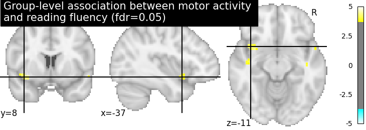
Let us plot the second level contrast at the computed thresholds

from nilearn import plotting
plotting.plot_stat_map(
    z_map, threshold=threshold, colorbar=True,
    title='Group-level association between motor activity \n'
    'and reading fluency (fdr=0.05)')

plotting.show()

Computing the (corrected) p-values with parametric test to compare with non parametric test

from nilearn.image import math_img
from nilearn.input_data import NiftiMasker
from nistats.utils import get_data

p_val = model.compute_contrast('fluency', output_type='p_value')
n_voxels = np.sum(get_data(model.masker_.mask_img_))
# Correcting the p-values for multiple testing and taking negative logarithm
neg_log_pval = math_img("-np.log10(np.minimum(1, img * {}))"
                        .format(str(n_voxels)),
                        img=p_val)

Out:

<string>:1: RuntimeWarning: divide by zero encountered in log10

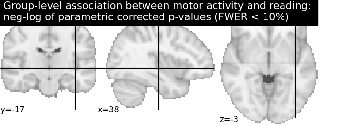
Let us plot the (corrected) negative log p-values for the parametric test

cut_coords = [38, -17, -3]
# Since we are plotting negative log p-values and using a threshold equal to 1,
# it corresponds to corrected p-values lower than 10%, meaning that there
# is less than 10% probability to make a single false discovery
# (90% chance that we make no false discoveries at all).
# This threshold is much more conservative than the previous one.
threshold = 1
title = ('Group-level association between motor activity and reading: \n'
         'neg-log of parametric corrected p-values (FWER < 10%)')
plotting.plot_stat_map(neg_log_pval, colorbar=True, cut_coords=cut_coords,
                       threshold=threshold, title=title)
plotting.show()

Computing the (corrected) negative log p-values with permutation test

from nistats.second_level_model import non_parametric_inference
neg_log_pvals_permuted_ols_unmasked = \
    non_parametric_inference(contrast_map_filenames,
                             design_matrix=design_matrix,
                             second_level_contrast='fluency',
                             model_intercept=True, n_perm=1000,
                             two_sided_test=False, mask=None,
                             smoothing_fwhm=5.0, n_jobs=1)

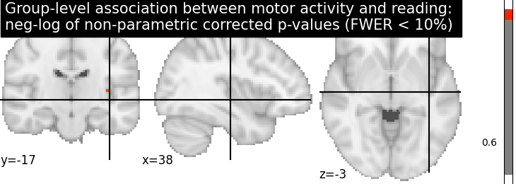
Let us plot the (corrected) negative log p-values

title = ('Group-level association between motor activity and reading: \n'
         'neg-log of non-parametric corrected p-values (FWER < 10%)')
plotting.plot_stat_map(neg_log_pvals_permuted_ols_unmasked, colorbar=True,
                       cut_coords=cut_coords, threshold=threshold,
                       title=title)
plotting.show()

# The neg-log p-values obtained with non parametric testing are capped at 3
# since the number of permutations is 1e3.
# The non parametric test yields a few more discoveries
# and is then more powerful than the usual parametric procedure.