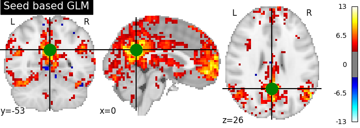
2.2.2. Default Mode Network extraction of AHDH dataset

This example shows a full step-by-step workflow of fitting a GLM to data extracted from a seed on the Posterior Cingulate Cortex and saving the results.

More specifically:

1. A sequence of fMRI volumes are loaded.

2. A design matrix with the Posterior Cingulate Cortex seed is defined.

3. A GLM is applied to the dataset (effect/covariance, then contrast estimation).

4. The Default Mode Network is displayed.

import numpy as np

from nilearn import datasets, plotting
from nilearn.input_data import NiftiSpheresMasker

from nistats.first_level_model import FirstLevelModel
from nistats.design_matrix import make_first_level_design_matrix

2.2.2.1. Prepare data and analysis parameters

Prepare the data.

adhd_dataset = datasets.fetch_adhd(n_subjects=1)

# Prepare timing
t_r = 2.
slice_time_ref = 0.
n_scans = 176

# Prepare seed
pcc_coords = (0, -53, 26)

Out:

/home/kshitij/miniconda3/envs/nistats-py36-latest/lib/python3.6/site-packages/nilearn/datasets/func.py:516: VisibleDeprecationWarning: Reading unicode strings without specifying the encoding argument is deprecated. Set the encoding, use None for the system default.
  dtype=None)

2.2.2.2. Estimate contrasts

Specify the contrasts.

seed_masker = NiftiSpheresMasker([pcc_coords], radius=10, detrend=True,
                                 standardize=True, low_pass=0.1,
                                 high_pass=0.01, t_r=2.,
                                 memory='nilearn_cache',
                                 memory_level=1, verbose=0)
seed_time_series = seed_masker.fit_transform(adhd_dataset.func[0])
frametimes = np.linspace(0, (n_scans - 1) * t_r, n_scans)
design_matrix = make_first_level_design_matrix(frametimes, hrf_model='spm',
                                               add_regs=seed_time_series,
                                               add_reg_names=["pcc_seed"])
dmn_contrast = np.array([1] + [0]*(design_matrix.shape[1]-1))
contrasts = {'seed_based_glm': dmn_contrast}

2.2.2.3. Perform first level analysis

Setup and fit GLM.

first_level_model = FirstLevelModel(t_r=t_r, slice_time_ref=slice_time_ref)
first_level_model = first_level_model.fit(run_imgs=adhd_dataset.func[0],
                                          design_matrices=design_matrix)

Out:

/home/kshitij/workspace/nistats-org/nistats-repo/nistats-kchawla-pi/nistats/first_level_model.py:73: UserWarning: Mean values of 0 observed.The data have probably been centered.Scaling might not work as expected
  warn('Mean values of 0 observed.'

Estimate the contrast.

print('Contrast seed_based_glm computed.')
z_map = first_level_model.compute_contrast(contrasts['seed_based_glm'],
                                           output_type='z_score')

# Saving snapshots of the contrasts
filename = 'dmn_z_map.png'
display = plotting.plot_stat_map(z_map, threshold=3.0, title='Seed based GLM',
                                 cut_coords=pcc_coords)
display.add_markers(marker_coords=[pcc_coords], marker_color='g',marker_size=300)
display.savefig(filename)
print("Save z-map in '{0}'.".format(filename))

Out:

Contrast seed_based_glm computed.
Save z-map in 'dmn_z_map.png'.

2.2.2.4. Generating a report

It can be useful to quickly generate a portable, ready-to-view report with most of the pertinent information. This is easy to do if you have a fitted model and the list of contrasts, which we do here.

from nistats.reporting import make_glm_report

report = make_glm_report(first_level_model,
                         contrasts=contrasts,
                         title='ADHD DMN Report',
                         cluster_threshold=15,
                         min_distance=8.,
                         plot_type='glass',
                         )

We have several ways to access the report:

# report  # This report can be viewed in a notebook
# report.save_as_html('report.html')
# report.open_in_browser()