2.2.3. Analysis of an fMRI dataset with a Finite Impule Response (FIR) model

FIR models are used to estimate the hemodyamic response non-parametrically. The example below shows that they’re good to do statistical inference even on fast event-related fMRI datasets.

Here, we demonstrate the use of a FIR model with 3 lags, computing 4 contrasts from a single subject dataset from the “Neurospin Localizer”. It is a fast event related design: During 5 minutes, 80 events of the following types are presented : [‘calculaudio’, ‘calculvideo’’, ‘clicDvideo’, ‘clicGaudio’, ‘clicGvideo’, ‘damier_H’, ‘damier_V’, ‘phraseaudio’, ‘phrasevideo’]

At first, we grab the localizer data.

import pandas as pd
from nistats import datasets

data = datasets.fetch_localizer_first_level()
fmri_img = data.epi_img
t_r = 2.4
events_file = data['events']
events = pd.read_table(events_file)

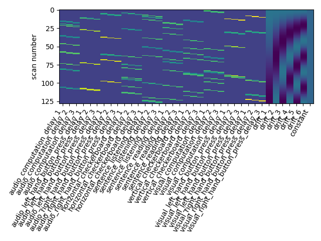
Next solution is to try Finite Impulse Reponse (FIR) models: we just say that the hrf is an arbitrary function that lags behind the stimulus onset. In the present case, given that the numbers of conditions is high, we should use a simple FIR model.

Concretely, we set hrf_model to ‘fir’ and fir_delays to [1, 2, 3] (scans) corresponding to a 3-step functions on the [1 * t_r, 4 * t_r] seconds interval.

from nistats.first_level_model import FirstLevelModel
from nistats.reporting import plot_design_matrix, plot_contrast_matrix

first_level_model = FirstLevelModel(t_r, hrf_model='fir', fir_delays=[1, 2, 3])
first_level_model = first_level_model.fit(fmri_img, events=events)
design_matrix = first_level_model.design_matrices_[0]
plot_design_matrix(design_matrix)

Out:

<matplotlib.axes._subplots.AxesSubplot object at 0x7f6ec426d0b8>

We have to adapt contrast specification. We characterize the BOLD response by the sum across the three time lags. It’s a bit hairy, sorry, but this is the price to pay for flexibility…

import numpy as np

contrast_matrix = np.eye(design_matrix.shape[1])
contrasts = dict([(column, contrast_matrix[i])
                  for i, column in enumerate(design_matrix.columns)])
conditions = events.trial_type.unique()
for condition in conditions:
    contrasts[condition] = np.sum(
        [contrasts[name] for name in design_matrix.columns
         if name[:len(condition)] == condition], 0)

contrasts['audio'] = np.sum([contrasts[name] for name in
                             ['audio_right_hand_button_press',
                              'audio_left_hand_button_press',
                              'audio_computation',
                              'sentence_listening']], 0)
contrasts['video'] = np.sum(
    [contrasts[name] for name in
     ['visual_right_hand_button_press',
      'visual_left_hand_button_press',
      'visual_computation',
      'sentence_reading']], 0)

contrasts['computation'] = contrasts['audio_computation'] +\
                           contrasts['visual_computation']
contrasts['sentences'] = contrasts['sentence_listening'] +\
                         contrasts['sentence_reading']

contrasts = {
    'left-right': (
        contrasts['visual_left_hand_button_press'] +
        contrasts['audio_left_hand_button_press'] -
        contrasts['visual_right_hand_button_press'] -
        contrasts['audio_right_hand_button_press']),
    'H-V': (contrasts['horizontal_checkerboard'] -
            contrasts['vertical_checkerboard']),
    'audio-video': contrasts['audio'] - contrasts['video'],
    'sentences-computation': (contrasts['sentences']-contrasts['computation'])
}

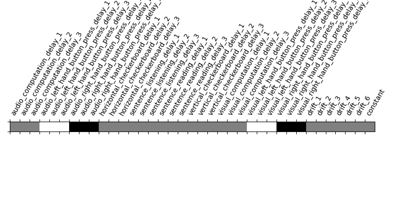
Take a look at the contrasts.

plot_contrast_matrix(contrasts['left-right'], design_matrix)

Out:

<matplotlib.axes._subplots.AxesSubplot object at 0x7f6ec409ad68>

Take a breath.

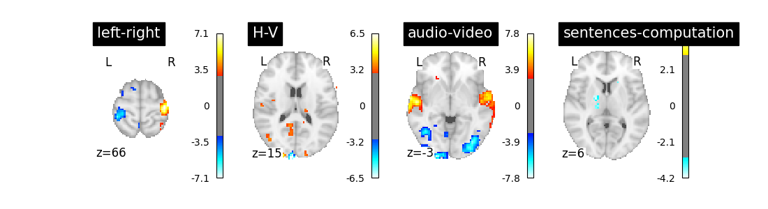
We can now proceed by estimating the contrasts and displaying them.

import matplotlib.pyplot as plt
from nilearn.plotting import plot_stat_map

fig = plt.figure(figsize=(11, 3))
for index, (contrast_id, contrast_val) in enumerate(contrasts.items()):
    ax = plt.subplot(1, len(contrasts), 1 + index)
    z_map = first_level_model.compute_contrast(
        contrast_val, output_type='z_score')
    plot_stat_map(
        z_map, display_mode='z', threshold=3.0, title=contrast_id, axes=ax,
        cut_coords=1)
    plt.show()

Out:

/home/kshitij/workspace/nistats-org/nistats-repo/nistats-kchawla-pi/examples/02_first_level_models/plot_fir_model.py:109: UserWarning: Matplotlib is currently using agg, which is a non-GUI backend, so cannot show the figure.
  plt.show()

The result is acceptable. Note that we’re asking a lot of questions to a small dataset, yet with a relatively large number of experimental conditions.