2.3.2. Second-level fMRI model: a two-sample test

Full step-by-step example of fitting a GLM to perform a second level analysis in experimental data and visualizing the results.

More specifically:

1. A sample of n=16 visual activity fMRIs are downloaded.

2. A two-sample t-test is applied to the brain maps in order to see the effect of the contrast difference across subjects.

The contrast is between responses to vertical versus horizontal checkerboards that are retinotopically distinct. At the individual level, these stimuli are sometimes used to map the borders of primary visual areas. At the group level, such a mapping is not possible. Yet, we may observe some significant effects in these areas.

import pandas as pd
from nilearn import plotting
from nilearn.datasets import fetch_localizer_contrasts

2.3.2.1. Fetch dataset

We download a list of left vs right button press contrasts from a localizer dataset.

n_subjects = 16
sample_vertical = fetch_localizer_contrasts(
    ["vertical checkerboard"], n_subjects, get_tmaps=True)
sample_horizontal = fetch_localizer_contrasts(
    ["horizontal checkerboard"], n_subjects, get_tmaps=True)

# What remains implicit here is that there is a one-to-one
# correspondence between the two samples: the first image of both
# samples comes from subject S1, the second from subject S2 etc.

Out:

/home/kshitij/miniconda3/envs/nistats-py36-latest/lib/python3.6/site-packages/numpy/lib/npyio.py:2372: VisibleDeprecationWarning: Reading unicode strings without specifying the encoding argument is deprecated. Set the encoding, use None for the system default.
  output = genfromtxt(fname, **kwargs)

2.3.2.2. Estimate second level model

We define the input maps and the design matrix for the second level model and fit it.

second_level_input = sample_vertical['cmaps'] + sample_horizontal['cmaps']

Next, we model the effect of conditions (sample 1 vs sample 2).

import numpy as np
condition_effect = np.hstack(([1] * n_subjects, [- 1] * n_subjects))

Subsequently, we can model the subject effect: each subject is observed in sample 1 and sample 2.

subject_effect = np.vstack((np.eye(n_subjects), np.eye(n_subjects)))
subjects = ['S%02d' % i for i in range(1, n_subjects + 1)]

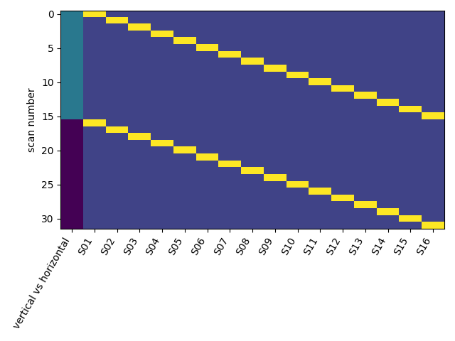
We then assemble those in a design matrix and

design_matrix = pd.DataFrame(
    np.hstack((condition_effect[:, np.newaxis], subject_effect)),
    columns=['vertical vs horizontal'] + subjects)

plot the design_matrix.

from nistats.reporting import plot_design_matrix
plot_design_matrix(design_matrix)

Out:

<matplotlib.axes._subplots.AxesSubplot object at 0x7f6ec4095438>

We formally specify the analysis model and fit it.

from nistats.second_level_model import SecondLevelModel
second_level_model = SecondLevelModel().fit(
    second_level_input, design_matrix=design_matrix)

Estimating the contrast is very simple. We can just provide the column name of the design matrix.

z_map = second_level_model.compute_contrast('vertical vs horizontal',
                                            output_type='z_score')

We threshold the second level contrast and plot it.

threshold = 3.1  # correponds to  p < .001, uncorrected
display = plotting.plot_glass_brain(
    z_map, threshold=threshold, colorbar=True, plot_abs=False,
    title='vertical vs horizontal checkerboard (unc p<0.001')

plotting.show()

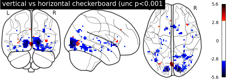
Unsurprisingly, we see activity in the primary visual cortex, both positive and negative.